Example: one HBN participant#
This example runs MPAT on real data: one participant of the Healthy Brain Network
Processed Open Diffusion Derivatives (HBN-POD2) [Alexander et al., 2017, Richie-Halford et al., 2022].
It follows pyAFQ’s tutorial
Getting started with pyAFQ – ParticipantAFQ
up to the ParticipantAFQ object. From there, MPAT replaces tractography and bundle
recognition.
The whole example is one script,
examples/hbn_participant.py:
pip install "pyAFQ[aws]"          # boto3, to download HBN-POD2 from its public S3 bucket
python examples/hbn_participant.py --n-proc 8 --max-mem 32GB
The data#
fetch_hbn_preproc downloads one subject’s qsiprep-preprocessed data, about 400 MB, and
organises it as BIDS derivatives under ~/AFQ_data/HBN/:
import os
import os.path as op

import AFQ.data.fetch as afd
import AFQ.definitions.image as afm
from AFQ.api.participant import ParticipantAFQ

afd.fetch_hbn_preproc(["NDARAA948VFH"])

sub_dir = op.join(afd.afq_home, "HBN", "derivatives", "qsiprep", "sub-NDARAA948VFH")
dwi = op.join(sub_dir, "ses-HBNsiteRU", "dwi",
              "sub-NDARAA948VFH_ses-HBNsiteRU_acq-64dir_space-T1w_desc-preproc_dwi")
anat = op.join(sub_dir, "anat", "sub-NDARAA948VFH")

output_dir = op.join(afd.afq_home, "HBN", "derivatives", "afq", "sub-NDARAA948VFH",
                     "ses-HBNsiteRU", "dwi")
os.makedirs(output_dir, exist_ok=True)
The pyAFQ participant#
As in the tutorial, the partial volume estimates (PVE) and the brain mask come from qsiprep. MPAT uses the PVE to decide where walkers move (white matter), where they end (grey matter), and where they never go (CSF). See the tissue table.
pve = afm.PVEImages(afm.ImageFile(path=f"{anat}_label-CSF_probseg.nii.gz"),
                    afm.ImageFile(path=f"{anat}_label-GM_probseg.nii.gz"),
                    afm.ImageFile(path=f"{anat}_label-WM_probseg.nii.gz"))
brain_mask_definition = afm.ImageFile(path=f"{anat}_desc-brain_mask.nii.gz")

myafq = ParticipantAFQ(
    dwi_data_file=f"{dwi}.nii.gz",
    bval_file=f"{dwi}.bval",
    bvec_file=f"{dwi}.bvec",
    t1_file=f"{anat}_desc-preproc_T1w.nii.gz",
    output_dir=output_dir,
    tracking_params=dict(odf_model="CSD"),
    pve=pve,
    brain_mask_definition=brain_mask_definition,
)
One difference from the tutorial: tracking_params only names the fODF model. pyAFQ’s
seeding options (n_seeds, random_seeds, rng_seed) do not apply, because MPAT does not
sample streamlines. It launches one streamline’s worth of walker mass from every voxel of
the white/grey-matter interface, and follows all of it exactly.
Running MPAT#
import mpat

results = mpat.run(myafq, n_proc=8, max_mem="32GB")      # -> <output_dir>/mpat/
mpat.run asks pyAFQ for what it needs:
the CSD fODF
the tissue PVE and the brain mask
the white/grey-matter interface, for the seeds
the registration to the template, to warp each bundle’s ROIs to the subject
It does not need pyAFQ’s tractography. It then builds the chain once and solves for every bundle in pyAFQ’s default bundle dictionary.
On this participant, with 8 threads:
white-matter voxels |
66,809 |
chain |
1,737,034 states (voxels × 26 direction classes), 94.9 million transitions, 1.0 GB, built in 19 s |
seeds |
23,801 interface voxels → 62,569 half-walk pairs (one streamline per seed, split over its fODF peaks) |
solves |
36 bundles in two groups of columns ( |
time |
17.6 minutes for MPAT. The first run also downloads the data and computes pyAFQ’s derivatives (DTI and CSD fits, registration): about 30 minutes in all |
Every bundle’s endpoint_mass_check is 1 to within \(10^{-5}\) (the largest deviation, \(7.5 \times 10^{-6}\), is for the bundle with the fewest expected streamlines, Callosum Temporal).
Results#
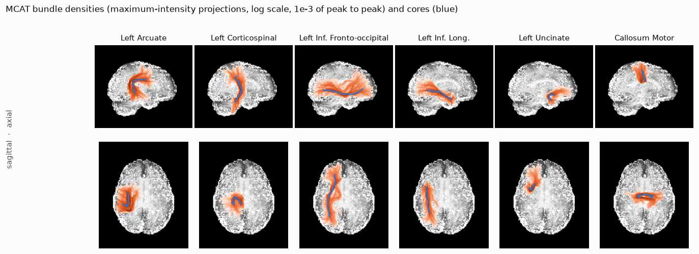
Figure 1 Six of the 36 bundles, as maximum-intensity projections of the density over FA, with each bundle’s core in blue. Images are shown in RAS orientation: the subject’s left is on the left of the axial views, anterior is up in the axial views, and anterior is to the right in the sagittal views. Each bundle’s density is drawn on its own log scale, from \(10^{-3}\) of its peak to its peak, so the panels show each bundle’s shape but not its absolute size; that is set by the expected streamline counts below.#
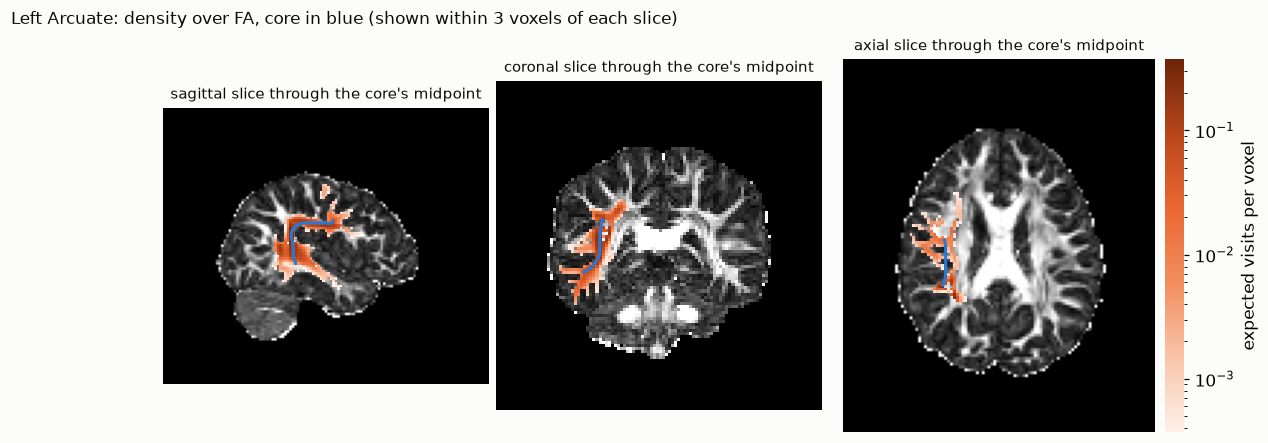
Figure 2 The left arcuate on three slices through the midpoint of its core: expected visits per voxel, over FA.#
Each bundle’s files are described in Outputs. The run’s table,
sub-NDARAA948VFH_ses-HBNsiteRU_acq-64dir_desc-mpat_table.tsv, lists every bundle:
Expected streamlines are counted out of the 23,801 seeds, one streamline per seed. Each count is the sum over seeds of the probability that the seed’s streamline meets the bundle’s definition. Columns is the number of solution columns the bundle needed: one per pair of avoid set (from its include ROIs) and end kind (from its endpoint ROIs).
bundle |
expected streamlines |
columns |
|---|---|---|
Left Optic Radiation |
0.55 |
8 |
Right Optic Radiation |
1.6 |
8 |
Left Anterior Thalamic |
0.88 |
8 |
Right Anterior Thalamic |
0.22 |
8 |
Left Cingulum Cingulate |
0.07 |
8 |
Right Cingulum Cingulate |
0.60 |
8 |
Left Corticospinal |
2.0 |
8 |
Right Corticospinal |
1.8 |
8 |
Left Inferior Fronto-occipital |
0.0024 |
8 |
Right Inferior Fronto-occipital |
0.08 |
8 |
Left Inferior Longitudinal |
0.48 |
8 |
Right Inferior Longitudinal |
0.90 |
8 |
Left Arcuate |
2.2 |
12 |
Right Arcuate |
16.8 |
12 |
Left Uncinate |
1.5 |
12 |
Right Uncinate |
9.0 |
12 |
Left Posterior Arcuate |
28.9 |
4 |
Right Posterior Arcuate |
37.6 |
4 |
Left Temporo-parietal |
1.2 |
8 |
Right Temporo-parietal |
0.51 |
8 |
Left Vertical Occipital |
183.7 |
12 |
Right Vertical Occipital |
265.9 |
12 |
Left Superior Longitudinal I |
10.7 |
8 |
Left Superior Longitudinal II |
18.8 |
8 |
Left Superior Longitudinal III |
22.6 |
8 |
Right Superior Longitudinal I |
5.2 |
8 |
Right Superior Longitudinal II |
15.2 |
8 |
Right Superior Longitudinal III |
32.0 |
8 |
Callosum Anterior Frontal |
11.8 |
8 |
Callosum Motor |
0.69 |
8 |
Callosum Occipital |
0.17 |
8 |
Callosum Orbital |
0.97 |
8 |
Callosum Posterior Parietal |
0.02 |
8 |
Callosum Superior Frontal |
2.0 |
8 |
Callosum Superior Parietal |
0.08 |
8 |
Callosum Temporal |
0.0017 |
8 |
The counts range over five orders of magnitude, from 266 for the right vertical occipital fasciculus to 0.002 for the callosal temporal bundle.
Looking at the bundles interactively#
In a notebook, mpat.view shows the densities, cores and visitation-ODF glyphs in NiiVue:
mpat.view(op.join(output_dir, "mpat"), bundles=["LeftArcuate", "LeftCorticospinal"], glyphs=True)
and mpat.save_html writes the same scene as one web page:
mpat.save_html("hbn_bundles.html", op.join(output_dir, "mpat"),
                      bundles=["LeftArcuate", "LeftCorticospinal"], glyphs=True)
The page for this run (left arcuate and left corticospinal, with glyphs) is here (1.6 MB; NiiVue loads from a CDN).
Going further#
moments=True(--momentsin the script) carries each walker’s sub-voxel position. Bundles come out narrower, at about 5× the run time (12. Spatial moments).bundles=[...](--bundlesin the script) segments only some of the bundles.