How MPAT works#
MPAT computes white-matter bundles as exact expectations over infinitely many streamlines. Instead of sampling streamlines and counting where they go, it writes probabilistic tracking as an absorbing Markov chain and solves that chain with linear algebra. This page walks through the method step by step.
Every figure on this page is computed by MPAT
The figures and animations run MPAT’s own code (mpat.Chain, mpat.segment_bundles,
mpat.bundle_core, …) on a small synthetic brain, the phantom in Figure 4.
It is one slice of 2 mm voxels with two crossing bundles: a U-shaped arc and a straight
stem. The scripts are in docs/animations/
and are re-run whenever MPAT’s source changes.
1. Tracking as a random walk, and its expectation#
Probabilistic tractography launches streamlines from seed points and lets each one take random steps, guided by the fibre orientation distribution (fODF). A bundle’s density map is then the expected number of steps that the bundle’s streamlines take in each voxel. Tracking software estimates that expectation from a finite sample of streamlines. The estimate is noisy, and the error falls only as \(1/\sqrt{N}\).
MPAT computes the expectation itself. The tracker’s state (where the walker is, and which way it is heading) evolves as a Markov chain. Grey matter, the edge of the brain mask, and dead ends are absorbing states, where a streamline stops. Expected visits and absorption probabilities in an absorbing chain have closed forms: the solutions of linear systems [Kemeny and Snell, 1960].
Figure 3 Monte Carlo tracking, sampled step by step from the same transition probabilities that MPAT
uses, converges to MPAT’s exact density. Its error falls as \(1/\sqrt{N}\), so 100,000
streamlines still leave about 2% error. MPAT has no sampling error; only the solver tolerance
remains (tol, default \(10^{-10}\)).#
2. Tissue, and the states of the chain#
MPAT takes all of its inputs from pyAFQ:
the fODF that pyAFQ’s tracker would follow
the tissue partial-volume estimates (PVE) and the brain mask
the seeds
the bundle definitions, with their ROIs warped to the subject
Each voxel inside the mask gets one of four roles, chosen as pyAFQ’s tracker chooses
(mpat.afq.tissue_labels):
tissue |
rule |
role in the chain |
|---|---|---|
white matter |
WM PVE > 0.4 |
transient: walkers move here |
grey matter |
otherwise, where GM PVE ≥ CSF PVE |
absorbing, a valid end |
CSF |
otherwise |
blocked: never entered; a hop into CSF has probability 0 |
edge |
the mask’s inner boundary |
absorbing, a valid end (fibres leaving the field of view) |
A walker on its way through white matter remembers which way it is going. A state of the chain is therefore a pair
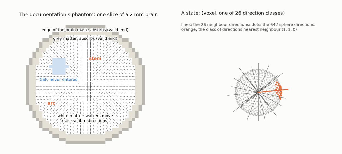
Figure 4 Left: the phantom, with tissue roles and the fibre direction in each white-matter voxel. Above and below the slice is CSF, which keeps every walker in the plane. Right: the 26 direction classes split the sphere’s 642 directions by their nearest neighbour direction.#
3. Hops inside a voxel (MITTENS)#
The geometry of a step comes from MITTENS [Cieslak et al., 2018]. A walker moves in
hops one voxel long (of the smallest voxel side), and each hop turns by less than the
maximum angle (angle, 35° by default) from the previous one. MITTENS enumerates every
sequence of hops \(p = (d_1, \dots, d_L)\) that a walker can take inside one voxel before it
leaves for one of the 26 neighbours. For each sequence it computes the exact volume of
start points \(\mathrm{vol}_p\) that realise it. The directions come from DSI Studio’s
642-direction sphere, and anisotropic voxels are handled exactly.
MPAT keeps two things from each path that MITTENS’s first-order model does not need:
its last hop’s direction class, which becomes the walker’s memory in the next voxel
its box of start points, which the spatial-moment closure uses (12. Spatial moments)
See mpat.geometry.build_geometry.
Figure 5 The start points of one voxel, all taking the same first hop. Start points that share a fate (the same hop sequence and the same exit neighbour) fill an axis-aligned box. MITTENS gives each box’s volume exactly, and the volumes tile the voxel. Start points whose first hop stays inside turn within the cone and hop again. With a uniform fODF, these volumes are the exit probabilities on the right.#
4. Transition probabilities#
Let \(X_v(d)\) be voxel \(v\)’s fODF on the sphere. It is clipped at zero, values below 5% of the maximum are zeroed (as in pyAFQ’s tracker), and it is normalised to sum to 1. Let \(Y_v(a)=\sum_{d\in\mathrm{cone}(a)}X_v(d)\) be its sum over the cone of directions within the turning angle of \(a\). A walker heading \(a\) turns to \(d\) with probability
A walker that enters voxel \(v\) heading \(e\) leaves it into neighbour \(n\), with last hop \(d_L\), with probability
\(L_n\) is the look-ahead. In doubleODF mode (the default, similar to iFOD2 [Tournier et al., 2010]), \(L_n(d_L)=Y_n(d_L)\): a hop is also weighted by how well the next voxel’s fODF supports it. In singleODF mode, \(L_n = 1\). Either way, \(L_n=0\) when \(n\) is CSF.
\(Z_v(e)\) normalises over every outcome. Hops into CSF get zero weight, so their probability is shared among the walker’s other hops.
If \(Z_v(e)=0\), the walker has no admissible continuation: it dies in white matter, which is not a valid end.
A state knows only the direction class \(b\), not the exact direction \(e\). Within its class, the incoming direction is spread as \(q_{v,b}(e) \propto X_v(e)\,Y_v(e)\). The state-to-state transition probability is then
mpat.kernel.chunk_blocks.
Figure 6 One voxel beside both bundles, read from the chain’s rows. A walker’s next voxel depends on its direction class: the state’s memory. singleODF follows this voxel’s fODF only. doubleODF also weighs each hop by the fODF of the voxel it lands in (grey glyphs). Heading north, the north-west neighbour, whose vertical lobe matches the walker’s direction, gains probability over the north neighbour, whose fibres run sideways.#
Storage
Which (neighbour, arrival class) pairs a class can reach is fixed by the geometry: about
150 of the 676 combinations. Each transition is therefore stored as a 1-byte slot into its
class’s template plus a float64 weight. One copy serves both directions: forward steps
scatter \(Q^\top x\), and backward steps gather \(Qx\) (mpat.chain.Chain).
5. The absorbing chain#
Order the states as white-matter (transient) states and absorbing voxels. One step of the chain is
\(N_{ij}\) is the expected number of visits to state \(j\) by a walker that starts in state \(i\).
\(NR\) gives the probabilities of where the walker ends.
MPAT never forms \(N\). It applies it to many vectors at once, as described below.
6. Seeds and launches#
Seeds are the white-matter voxels on the white/grey-matter interface (pyAFQ’s
wm_gm_interface). Each seed contributes one streamline, split evenly over the fODF
peaks found by DIPY’s peak finder with pyAFQ’s thresholds (relative 0.25, at least 45°
apart). A streamline along peak \(p\) is two half-walks: one launched along \(+p\) and one
along \(-p\). Each half’s first exit from the seed voxel uses the same path sums, with the
incoming direction fixed to the peak (mpat.prepare_launches).
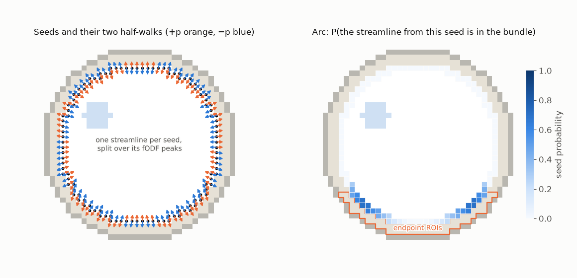
Figure 7 Left: the phantom’s seeds and the two half-walks of each streamline. Right: for the arc
bundle (end in each foot), the probability that the streamline from each seed belongs to the
bundle. This is MPAT’s seedprob output.#
7. Forward pass: where the walkers go#
Put every half-walk’s launch distribution into one vector \(\pi_0\). The expected number of visits to every state, by every walker from every seed, is
tol (default
\(10^{-10}\)), relative to the starting mass. A typical bundle loses about 10% of its mass per
step, which takes 300–500 steps.
If the remaining mass decays so slowly that power iteration would need 500 or more further
steps, or stalls (walkers circling in nearly all-white-matter volumes), the rest of the series
is solved as one linear system with BiCGSTAB [van der Vorst, 1992]
(mpat.solve.solve_series).
Figure 8 The forward pass on the phantom, one product with \(Q^\top\) per step. Half of the mass ends
at once: an interface seed’s outward half-walk steps straight into grey matter. The rest
crosses the white matter, never enters the CSF, and is absorbed at the far side. The mass
still moving falls below tol in about 66 steps, with no sampling.#
8. Backward pass: who completes the bundle#
A bundle needs more than reaching some grey matter. Its streamlines must end in particular places and pass through, or avoid, particular ROIs. Write \(r\) for the probability of being absorbed, in one step, somewhere the requirement accepts. The probability that a walker in state \(s\) eventually meets the requirement is then
Figure 9 The backward pass for “ends in the arc’s end ROI”. The completion probability \(\beta\) spreads back from the ROI one step at a time. Right: \(\beta\) depends on the direction class. Near the ROI, walkers heading toward it complete with probability near 1, and walkers heading away almost never do.#
9. Bundle density: occupancy × completion#
A visit to state \(s\) belongs to a bundle streamline when two things hold:
the walker got to \(s\), and its partner half met its own requirement (the forward pass, with the launch of each half weighted by its partner’s completion probability);
from \(s\), the walker goes on to meet its requirement (the backward pass).
These are independent given the state, because the chain is Markov. The bundle’s expected visits to \(s\) are therefore
Figure 10 The arc bundle as the product of the two passes, both filling in step by step. Left: occupancy of the half-walks whose partner ended in the start ROI. Middle: each state’s probability of ending in the end ROI. Right: their product, summed per voxel, is this half’s share of the bundle. Adding the mirror image (the half that ends in the start ROI) gives the bundle’s density.#
10. ROIs#
pyAFQ’s bundle definitions are turned into requirements on the two halves of a streamline
(mpat.afq.bundle_specs). What each kind of ROI means in practice, and MPAT’s additions to
pyAFQ’s definitions, are in Bundle definitions: include, exclude and endpoint ROIs.
Exclude ROIs make states taboo. A walker that enters a taboo voxel is removed from the column; in the solves, that is a diagonal mask \(M\):
mpat.afq.seal_26), so
that walkers stepping diagonally cannot slip through it.
Include ROIs need inclusion–exclusion, because “passes through A” is not something a mask can express. “Passes through A and B” is turned into a signed sum of avoidance problems, each of which is an exclusion:
Figure 11 Two include ROIs, A and B, one on each limb of the arc. Each of the four terms is the density of an exclusion problem, one solution column. The signed running sum overshoots (blue is negative), then settles on the walkers that pass through both ROIs.#
Endpoint ROIs are handled by end kinds. Every streamline has two ends, so the event “both ends are valid, and at least one is in the endpoint ROI” is a bilinear form in the two halves’ completion probabilities:
ROIs |
end kinds \(k\) |
\(M\) |
|---|---|---|
none |
valid (grey matter or edge) |
\((1)\) |
one endpoint ROI \(E\) |
valid; valid and not in \(E\) |
\(\mathrm{diag}(1, -1)\) |
start \(S\) and end \(E\) |
in \(S\); in \(E\) (and in both, if they overlap) |
swaps \(S \leftrightarrow E\), minus the double count |
Endpoint ROIs are grown by pyAFQ’s dist_to_atlas before use. pyAFQ’s other criteria
(curvature, length, cleaning) are defined on individual streamlines, so they do not apply.
11. Many bundles in one solve#
Each pair (avoid set, end kind) is one column: one backward and one forward series.
All columns move through the same products with \(Q\) and \(Q^\top\), so MPAT solves many
columns, and many bundles, in a single pass over the transition matrix. Bundles are packed in
order into groups whose columns fit in max_mem, at about \(12 \times 8\) bytes per state per
column at the peak (mpat.solve.max_columns). A bundle with two include ROIs and start/end
ROIs needs \(2^2 \times 2 = 8\) columns.
12. Spatial moments#
The chain as described forgets where inside a voxel a walker is. Every voxel restarts its paths from a uniform distribution of start points. For a bundle that runs obliquely to the grid, this adds lateral spread at every step, and bundles come out several times too wide.
With moments=True, each state also carries the walker’s mean sub-voxel position: \((M, Q)\)
with \(Q = M\bar{x}\) (voxel units, from the centre). Within the voxel, the density is
reconstructed linearly, \(\rho(y) = 1 + 12\,Q\cdot y / M\) [Prather, 1986]. Each
MITTENS path has a box of start points (centre \(c\), widths \(w\)) and lands at \(l\) in the next
voxel. Given \(x = Q/M\), the path then carries exactly
It is not positivity-preserving: masses can go slightly negative.
A few loops of states can amplify.
mpat.moments.stabilizefinds them by power iteration and falls back to the uniform closure in the voxels that carry them.It is about 5× slower.
Figure 12 A unit of walker mass launched along an oblique fibre (18° to the grid). Top: with a uniform restart in every voxel, the mass spreads sideways. Bottom: carrying the mean sub-voxel position keeps it on the fibre. Right: the cross-section at the blue line is about 2.5× narrower with moments (SD 1.06 vs 2.54 voxels).#
13. What comes out#
From \(S\), \(\beta\), and the absorbed mass, MPAT writes the following (see Outputs):
Density. The expected steps of bundle streamlines in each voxel, summed over all seeds.
Endpoints. The expected bundle endpoints in each grey-matter or edge voxel, two per streamline. Their total equals twice the expected number of bundle streamlines; the
endpoint_mass_checkin each summary file checks this.Seed probability. The probability that the streamline from each seed belongs to the bundle.
Visitation ODFs. The density kept per direction class, spread over the sphere within each class as the chain assumes (\(q\propto XY\)), symmetrised, and fitted with spherical harmonics in the fODF’s basis (lmax 8). Units are expected visits per steradian, so a voxel’s ODF integrates to its density. Where bundles cross, each bundle’s ODF keeps only the lobe its own walkers use.
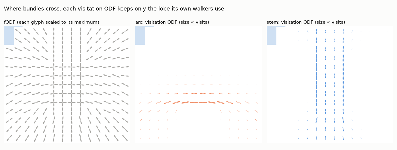
Figure 13 At the crossing, the fODF has both lobes. The arc’s visitation ODF keeps the horizontal lobe, and the stem’s keeps the vertical one.#
Core. A single curve along the bundle’s density ridge, 100 nodes long (
mpat.bundle_core). It is found in five steps:Anchor each end at the endpoint-weighted centre of its endpoints.
Find a most-probable path with Dijkstra and cost \(-\log(\text{density}/\text{peak})\) per mm. This finds the right corridor but cuts corners.
Assign every voxel to the cross-section of the nearest voxel on that path.
Run Dijkstra again with cost \(-\log(\text{density} / \text{its cross-section's maximum})\). This cost is zero along the ridge, so the path follows bends without a length penalty.
Smooth the path and resample it.
Figure 14 bundle_core stage by stage on the arc bundle.#
14. Checks#
Monte Carlo agreement. Figure 3, and the test suite (
tests/test_docs_phantom.py), check that sampled streamlines converge to MPAT’s density.Mass balance. Each bundle’s
*_desc-summary.jsonreportsendpoint_mass_check, which should be 1.Clipping. It also reports
negative_mass_before_clip, which is nonzero only with moments, and the iterations, Krylov products and final residual of both passes.
Works cited on this page are listed in References.